Story
Grism spectra need to be flat fielded in order to account for the differences in response of the pixels on the detector. The flat field cube method is complex and cumbersome and maybe not be even entirely correct. So this is a way to simplify flat-fielding of grism spectra.
Inputs
- A grism image
- A broadband flat field for the filter that is closest in wavelength coverage to the grism (e.g., F105W flat for the G102 grism, F140W for the G141 grism, F814W for the G800L grism).
Outputs
- A grism image
Computations
- Divide the grism image by the flat field.
Drawbacks
The following text is from Brammer et al. (2012), Appendix 1:
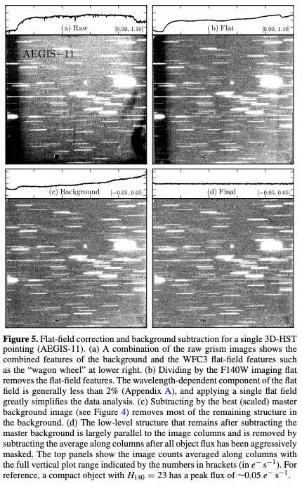
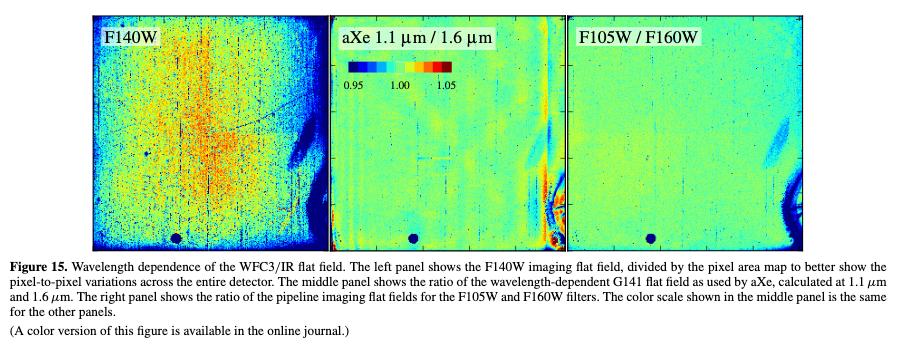
"Each pixel in a grism image “sees” the superposition of flux at different wavelengths coming from nearby positions on the sky where the grism disperses the flux to fall on top of that pixel. The standard aXe data reduction tries to account for this by applying a wavelength-dependent flat-field correction to pixels within the dispersed spectrum of a given object. We adopt a more simplified treatment of the flat field by simply dividing by the F140W imaging flat before the background subtraction and spectral extraction (Section 3.2.2). In doing so, we also separate multiplicative flat-field and additive background terms from the background subtraction. However, this technique ignores any wavelength dependence of the flat field, which is shown in Figure 15. The left panel of Figure 15 shows the F140W flat itself, with the large-scale variation resulting from the variable pixel areas (link is now broken) removed for display purposes. The middle panel shows the estimated ratio of the flat field at the blue to red edges of the G141 sensitivity, computed from the wavelength-dependent flat-field images used by aXe. The right panel of Figure15 shows the ratio of the pipeline imaging flats for the F105W and F160W filters. For both estimates, the wavelength dependence of the flat field across the G141 sensitivity is generally less than ±1% outside of the “wagon-wheel” feature in the lower right corner of the detector. The color dependence of the aXe flat field includes some high-frequency structure not seen in the ratio of the imaging flats and also appears to underestimate the decreased sensitivity in the wagon wheel at blue wavelengths. Our simplified treatment of dividing by the single F140W flat field can therefore result in flat-field errors of ∼5% in this part of the detector; however, dividing by this “average” flat is generally sufficient to flatten the background and reduce systematic effects caused by the background subtraction (see Figure 5)."
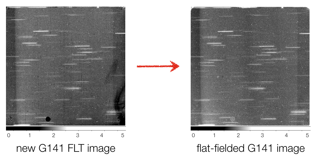
And a simple demo of an FLT before and after the flat-field division:
The main draw-back is that it's likely not quite right but we have never estimated exactly how wrong it is, if it is wrong in particular parts of the image and/or for particular SEDs. The only "hunch" we have that this is not quite right is that when we compare the slopes of grism spectra with the slopes of the SEDs in the same wavelength region, we find discrepancies. We correct for this in 3D-HST and in CLEAR. This could be caused by two compounding factors, the first is the flat-fielding and the second is the fact that we do not model the PSF variation as a function of wavelength. We have a ton of information (we save the slope corrections) that can in principle be used to figure this out but have not done it.