PS1-PSC: Probabilistic Classifications of Unresolved Point Sources in PanSTARRS1
A relatively new approach to star-galaxy separation is the classification table derived by Tachibana & Miller (2018, PASP 130, 995). The authors combined multiple sources of information from the PS1 databases (including the approaches described below) using a sophisticated machine-learning algorithm to estimate the point-source probabilities for 1.5 billion objects. The resulting table is accessible in MAST Casjobs in the HLSP_PS1_PSC database. It can be joined with the standard PS1 tables to get accurate classification probabilities for most objects in PS1. Here is an example Cajobs query that selects objects within 1 arcmin of RA=10 deg, Dec=20 deg:
-- Run this in the PanSTARRS_DR2 Casjobs context

select psc.objid, psc.ps_score, o.nDetections, o.nStackDetections
from fGetNearbyObjEq(10.0, 20.0, 1.0) f
join ObjectThin o on o.objid=f.objid
join HLSP_PS1_PSC.pointsource_scores psc on psc.objid=f.objid
See the PS1-PSC High Level Science Product page and the published paper for more details. We have seen good results using this data to separate blended and unblended stars in crowded regions in the Galactic plane.
PSF-Kron
The simplest way is to use the difference between PSFMag and KronMag. This has the advantage that it is available for all objects in the survey and in all the main tables.
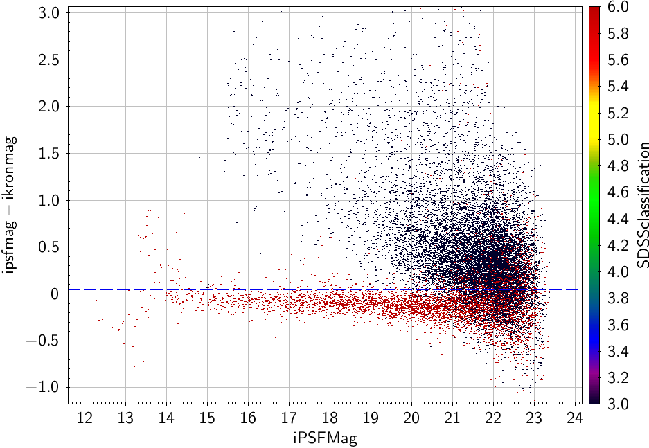 | This example is from a stack sample around Abell 1656 matched to SDSS and coloured by SDSS classification (red - stars; black - galaxies). A cut in iPSFMag-iKronMag of 0.05 (shown) does a reasonable job of separating stars and galaxies. |
|---|
You can calculate this using data from the MeanObject, StackObjectThin or ForcedMeanObject tables. You might improve the separation by combining results from more than one band or using a more sophisticated cut. Note that we do not expect PSF-Kron to be exactly 0.0 for stars, as Kron magnitudes by definition require a correction to take them to total magnitudes.
Faintward of i ~21 this simple cut becomes unreliable (usually over-predicts the number of stars). Also be aware that once stars become saturated (brighter than i ~14 in this example) they shift to the galaxy side of the cut. A full discussion of this method applied to Pan-STARRS data can be found in Farrow et al. (2014).
psfLikelihood
StackObjectAttributes (or StackObjectView) has a quantity psfLikelihood for each filter. This is around 0 for galaxies but can be either +1 or - 1 for stars. The best way to see what is happening is to plot a quantity like log10(abs(psfLikelihood))
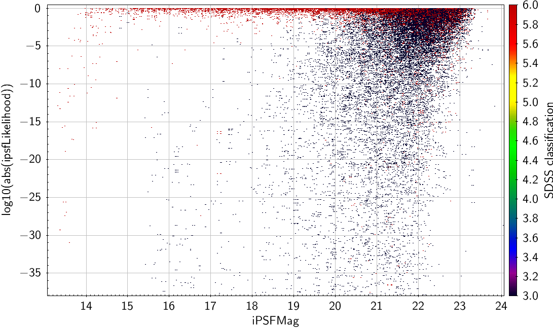 | Same sample as above, but now using log10(abs(ipsfLikelihood)) as the separator. |
|---|
Moments
Either momentsR1 or KronRad can be used as a separator (KronRad is 2.5*momentsR1 so it doesn't matter which you use)(again from StackObjectAttributes or StackObjectView).
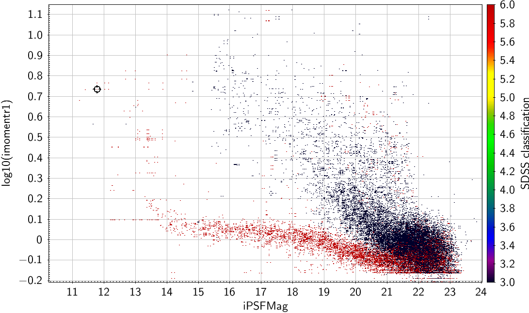 | Same sample as above, now using log10(imomentR1) as the separator. |
|---|
You can also try momentRH, which is the NOT the half light radius, but the expectation value of r^0.5 (again from StackObjectAttributes or StackObjectView) .
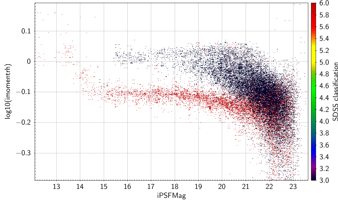 | Same sample as above, but now with log10(imomentRH) as the separator. |
|---|
Lensing parameters
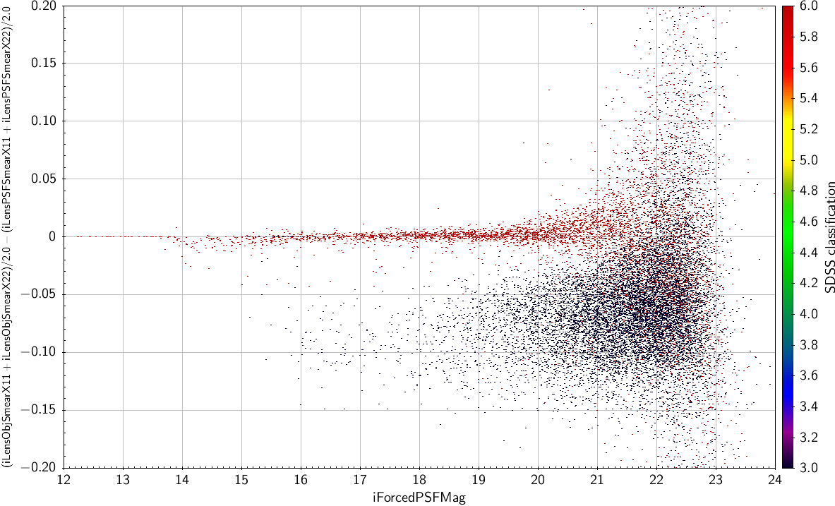
Another possibility is to use the lensing parameters, and try and make something which is not affected by seeing . These are found in the ForcedMeanLensing table. As an example, here is (iLensObjSmearX11+iLensObjSmearX22)/2.0 - (iLensPSFSmearX11+iLensPSFSmearX22)/2.0
| The combination of lensing parameters suggested in the text as a function of forced iPSF mag (from ForcedMeanObject) |
|---|
Other suggestions
The various model fits (Sersic, Exp, deVauc, Petrosian) also have radii associated with them, so you could try using mag v log(radius) for these, but remember they are not available for all objects.