FIMS-SPEAR observed the sky by rotating a spacecraft axis. The field of view, always moving with respect to celestial coordinates, swept across the sky. Thus, exposure time at a position on the sky cannot be understood as a difference between observation start and end times, as it can be understood for usual astronomical instruments. Instead, the teams first produced "virtual exposure events" (referred to as "exons"), and integrated the exons to make exposure maps.

FIMS Procedure

Exposure time for a point source

First, consider a simple limiting case of calculating the exposure time for a point source.

1. Suppose that the field of view crosses a point A on the sky at a given time t with an angular velocity V.
2. Then, the exposure time for the point A is given by the time interval needed for the slit angular width δθ₀ to cross point A. In other words, the exposure time is the crossing time, given by δθ₀/V.
3. The total exposure time for point A can then be calculated as follows:
   1. Find all time intervals during which point A was crossed.

   2. Calculate the angular velocities at the times that point A (with the size of a point spread function) is crossed, from the attitude information in the telemetry.
      

   3. Total exposure time for the point source is given by $\sum\limits_{i}\left(\delta\theta_0/V_i\right).$

Exposure map

The above method, however, is appropriate only for calculating the exposure time for a point source. A more useful definition of exposure time is as follows.

Consider, first, a brief moment in time as the FOV sweeps over the sky:

1. Consider a very short, fixed time interval δt = 0.1 seconds during which the location of the slit may be considered to be fixed in the sky. (The interval at which FIMS_TIME was measured, 0.1 seconds, was adopted for this time step δt.)

2. During the time interval δt, all points (e.g., A,B,C,... in Figure 1) in the field of view (FOV) will have the same exposure time δt.
   

   
   

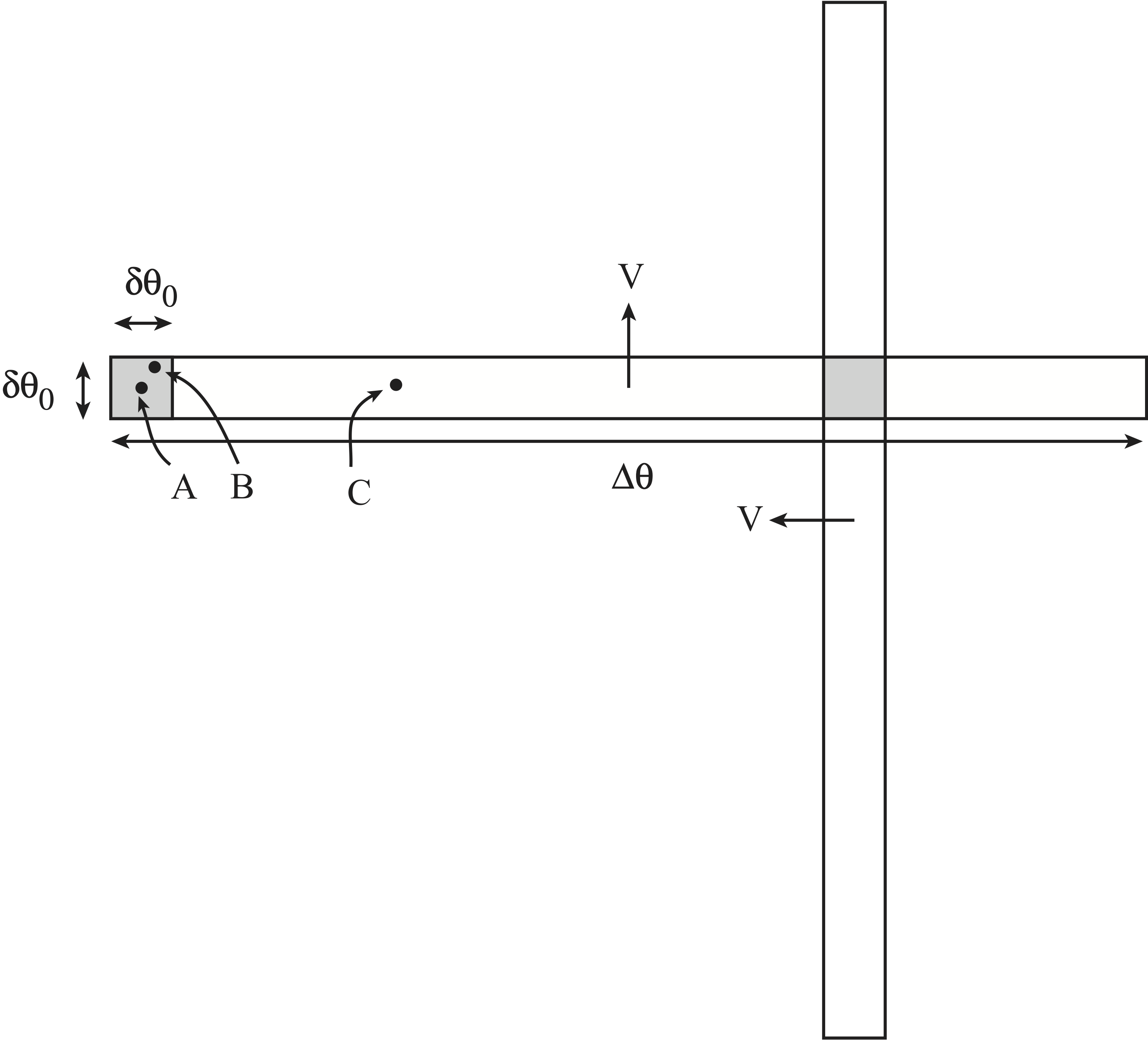
   Figure 1: Schematic diagram to calculate exposure time. Here, δθ₀ is the slit angular width and ∆θ is the view angle perpendicular to the slit’s long axis. V is the drift angular velocity of the FOV.

    

3. δt = 0.1 seconds later, the FOV center now points to a new position on the sky. This position is different from the center of the first FOV, but still overlaps with the first FOV. The region of overlap between the two FOVs now has an exposure time 2δt.

Thus, an exposure map can be constructed by assigning an exposure time event (corresponding to δt = 0.1 seconds) to every pixel with angular size (δθ₀)² within the FOV at a particular time t, and then counting the number of exposure time events contained in each unit pixel. These exposure time events are called exons. So, conceptually, the method is as follows:

1. Generate $N_0$ exposure events uniformly-distributed along the slit's long axis for each time step $\delta t$. (The available times steps were obtained from FIMS_TIME RECORD telemetry data.) These exons have angular coordinates $\phi_i = (i-1/2)\times(\phi_{\rm max}-\phi_{\rm min})/N_0 + \phi_{\rm min}$ (for $i=1,\cdots,N_0$). They do not have a wavelength coordinate. The exons have the quaternion as provided by the attitude files.

2. The angular distance along which the FOV moves perpendicular to the slit’s long axis during the time step δt is given by V δt.

3. Thus, the number of the exposure events for a unit pixel with an angular size of (δθ₀)² is given by
   

   $N=\left(\dfrac{\delta\theta_0}{V\delta t}\right)\left(N_0\dfrac{\delta\theta_0}{\Delta\theta}\right)$
   Here, $\Delta\theta=\phi_{\rm max}-\phi_{\rm min}$ and $N_0(\delta\theta_0/\Delta\theta)=1$ if only one exon per a unit pixel is generated along the slit's long axis.

4. Then, the exposure time for a unit pixel is obtained to be:
   

   $\dfrac{\delta\theta_0}{V}=\left(N\delta t\right) /\left(N_0\dfrac{\delta\theta_0}{\Delta\theta}\right).$

In practice, the pipeline carried out this methodology with the following steps:

1. Generate N₀ exons, uniformly-distributed over the imaging axis φ-angles, for every time step δt. Larger N₀ results in a smoother exposure map, but the computational requirements also become more memory-intensive.
   

2. Tag attitudes or coordinates (RA, DEC or Galactic longitude, latitude) to the generated exons.

3. Make an image that maps the total exon counts on the sky, binning the exons with an arbitrary sky pixel size of (δθ)² (corresponding to the size of pixels in the final products).

4. Multiply the generated image by a factor $\delta t/\left(N\dfrac{\delta \theta_0}{\Delta\theta}\right)$
5. The final exposure map is then obtained by scaling the image by $\left(\dfrac{\delta\theta_0}{\delta\theta}\right)^{2}$ $(=1$ if $\delta\theta=\delta\theta_0$).

The end result is a map in which values indicate the average exposure time per slit width² within that pixel.

FIMS vs. SPEAR Procedure

The SPEAR team's procedure, which has not been documented in detail, was conceptually similar. The two team's procedures differed from each other in the following respects:

• Instead of the FIMS etendue defined for a solid angle of δθ₀² (i.e., slit width squared), the SPEAR team used a similarly-sized etendue of δθ₀ x 5 arcmin. This distinction does not affect the data products provided at MAST, due to the next point.
  
• The FIMS team scaled by δθ₀²/δθ² to create the exposure map, while the SPEAR team did not include this conversion factor.
  • FIMS exposure map values indicate the average "exposure time per slit width squared" within each HEALPixel (in other words, exposure time per δθ₀²).
  • SPEAR exposure map values indicate summed exposure time per HEALPixel in the final products (in other words, exposure time per δθ², or the total amount of time the instrument spent collecting photons in that pixel).
• Thus, the typical exposure time value indicated by a FIMS exposure map pixel is independent of the map's spatial resolution, while the typical exposure time value indicated by a SPEAR exposure map pixel increases at lower spatial resolutions (scaling as HEALPixel Nside^-2, adding neighboring pixels together).
• The photon count maps for both SPEAR and FIMS indicate total count per pixel (i.e., counts per δθ²).
• Accordingly, in order to calculate the final intensity maps, the teams' procedures differed slightly:
  
  • The FIMS team divided the count map by the exposure map, then divided by their effective area curve from Effective Area | Grasp.
  • The SPEAR team divided the count map by the exposure map, then divided by their grasp curve from Effective Area | Grasp. Grasp is equal to effective area times FOV.
• Intensity is defined identically for both team's products; differences between the intensity maps are due to differences in other aspects of the data processing unrelated to exposure time.

Exposure Times in FITS Headers and Cross-Mission MAST Services

Because the FIMS team's definition of "exposure time" (exposure time per slit width squared) is independent of the post-processing spatial resolution of the final map, it is preferable as a means of comparing the exposure times of different products. The median value of this exposure time in a given file is provided in the FITS header as the keyword EXP-SLIT. For SPEAR products, MAST has calculated both the FIMS definition of exposure time (EXP-SLIT) and the SPEAR definition of exposure time (EXP-PIX). EXP-SLIT is used in cross-mission services such as the MAST Portal.

Supplementary Script Notes

Note: MAST does not currently provide the files described here. This section is provided verbatim from the FIMS team's notes to shine further light on how the higher-level products MAST does provide were produced, and for reference by the mission teams and their interlocutors.

1. FIMS exposure events have the naming convention as follows:

   1. fims orbit yyyy mm dd lexp.fits for L-band events

   2. fims orbit yyyy mm dd sexp.fits for S-band events

2. Data location: /fims/fims/FIMS_exon in space01.kasi.re.kr and in spacezero.kaist.ac.kr

3. Header keywords

   1. SLTWIDTH = δθ₀ = slit width in degree (4.3′ for L-band, 4.6′ for S-band)

   2. FILTER = filter (shutter) mode % (1, 0.1, and 0.01 for 100%, 10%, and 1%, respectively)

   3. WEIGHT = $\delta t/\left(N_0\dfrac{\delta\theta_0}{\Delta\theta}\right)$ = exposure time assigned to an individual exposure event (exon).

   4. WEIGHT2 = FILTER × WEIGHT × (SLTWIDTH)²

4. How to make an exposure-corrected photon-count image:

   1. Make a photon-count image (2-dimensional histogram, N(x,y)) with an arbitrary pixel size (δθ)², using a photon event file.

   2. Make an exon-count image (2-dimensional histogram, E(x, y)) with the same pixel size (δθ)², using a corresponding exon file.

   3. Exposure map $\varepsilon (x,y)$ can be obtained by multiplying a factor, FILTER $\times $ WEIGHT $\times $ $\left(\dfrac{\text{SLTWIDTH}}{% \delta\theta}\right)^{2}$= WEIGHT2 $\times $ $\left(\dfrac{1}{\delta \theta }\right)^{2},$ to the exon-count image, i.e., $\varepsilon (x,y)=E(x,y)\times{\rm WEIGHT2}\times\left(\dfrac{1}{\delta\theta}\right)^{2}$. Note that $\delta\theta$ should be in degree unit.

   4. The exposure-corrected photon-count image is then calculated by dividing the photon count image by the exposure map, and has a unit of counts/s/(pixel size)/(wavelength bandwidth).

   5. Intensity image, which is defined by $I(x,y)=\left[ N(x,y)/(\delta \theta)^{2}\right] /\varepsilon (x,y)/\delta\lambda$, is now given by $% I(x,y)=N(x,y)/E(x,y)$/WEIGHT2/$\delta \lambda$. The intensity map has a unit of counts/s/degree$^{2}$/Å.